Unknown Facts About Vlookup Excel

By pushing ctrl+change+center, this will certainly calculate and return worth from numerous ranges, instead of simply private cells contributed to or increased by each other. Calculating the sum, item, or ratio of specific cells is very easy-- just utilize the =SUM formula as well as go into the cells, worths, or array of cells you want to perform that arithmetic on.

If you're looking to discover overall sales earnings from a number of marketed units, for example, the range formula in Excel is perfect for you. Right here's how you 'd do it: To start utilizing the array formula, type "=AMOUNT," and in parentheses, get in the first of two (or 3, or 4) arrays of cells you wish to multiply together.

This means multiplication. Following this asterisk, enter your second range of cells. You'll be multiplying this second variety of cells by the very first. Your development in this formula should currently resemble this: =SUM(C 2: C 5 * D 2:D 5) Ready to push Get in? Not so fast ... Since this formula is so difficult, Excel reserves a different keyboard command for ranges.

This will identify your formula as an array, wrapping your formula in support personalities and also efficiently returning your item of both arrays incorporated. In revenue estimations, this can reduce your time and also initiative dramatically. See the final formula in the screenshot above. The MATTER formula in Excel is represented =MATTER(Start Cell: End Cell).

For example, if there are 8 cells with gotten in values in between A 1 and also A 10, =MATTER(A 1: A 10) will certainly return a worth of 8. The COUNT formula in Excel is especially beneficial for big spread sheets, wherein you want to see exactly how several cells include actual entrances. Do not be fooled: This formula won't do any type of math on the values of the cells themselves.

5 Simple Techniques For Interview Questions

Utilizing the formula in bold above, you can conveniently run a matter of active cells in your spreadsheet. The result will look a something like this: To do the typical formula in Excel, go into the worths, cells, or range of cells of which you're calculating the standard in the format, =STANDARD(number 1, number 2, etc.) or =AVERAGE(Beginning Worth: End Value).

Finding the standard of a range of cells in Excel keeps you from needing to locate specific amounts and afterwards performing a different department equation on your total amount. Utilizing =AVERAGE as your initial text entrance, you can allow Excel do all the benefit you. For referral, the average of a team of numbers amounts to the sum of those numbers, split by the number of items because team.

This will return the sum of the worths within a wanted variety of cells that all satisfy one standard. For instance, =SUMIF(C 3: C 12,"> 70,000") would return the amount of worths between cells C 3 and also C 12 from only the cells that are better than 70,000. Let's state you want to figure out the profit you created from a list of leads that are related to details location codes, or determine the sum of particular workers' salaries-- however only if they drop over a particular amount.

With the SUMIF feature, it does not have to be-- you can conveniently build up the amount of cells that fulfill certain criteria, like in the wage instance above. The formula: =SUMIF(range, criteria, [sum_range] Array: The variety that is being evaluated utilizing your requirements. Criteria: The requirements that establish which cells in Criteria_range 1 will be totaled [Sum_range]: An optional variety of cells you're mosting likely to accumulate in addition to the initial Variety entered.

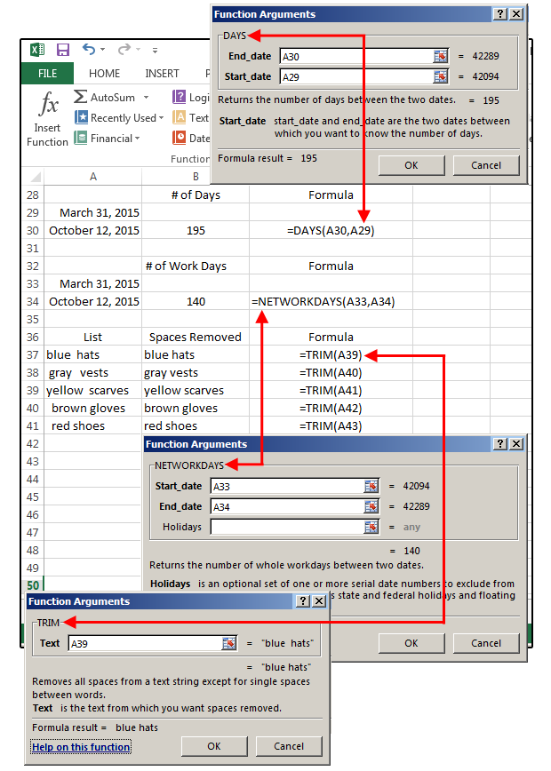
In the example listed below, we wanted to compute the amount of the salaries that were more than $70,000. The SUMIF function accumulated the dollar quantities that went beyond that number in the cells C 3 with C 12, with the formula =SUMIF(C 3: C 12,"> 70,000"). The TRIM formula in Excel is signified =TRIM(message).

A Biased View of Countif Excel

For instance, if A 2 includes the name" Steve Peterson" with unwanted areas prior to the initial name, =TRIM(A 2) would return "Steve Peterson" with no spaces in a brand-new cell. Email as well as submit sharing are remarkable tools in today's work environment. That is, until one of your associates sends you a worksheet with some truly cool spacing.

As opposed to painstakingly removing and including rooms as required, you can cleanse up any type of irregular spacing utilizing the TRIM function, which is used to remove extra spaces from data (besides solitary rooms in between words). The formula: =TRIM(message). Text: The message or cell from which you intend to remove spaces.

To do so, we went into =TRIM("A 2") into the Formula Bar, and replicated this for every name below it in a new column next to the column with undesirable areas. Below are some other Excel formulas you might find valuable as your information monitoring needs grow. Let's say you have a line of message within a cell that you wish to damage down right into a couple of different segments.

Purpose: Made use of to remove the very first X numbers or characters in a cell. The formula: =LEFT(message, number_of_characters) Text: The string that you desire to draw out from. Number_of_characters: The variety of personalities that you want to draw out beginning with the left-most personality. In the instance listed below, we got in =LEFT(A 2,4) right into cell B 2, and also duplicated it into B 3: B 6.

Function: Made use of to extract personalities or numbers in the center based upon placement. The formula: =MID(text, start_position, number_of_characters) Text: The string that you desire to remove from. Start_position: The position in the string that you intend to begin extracting from. As an example, the initial setting in the string is 1.

The Single Strategy To Use For Excel Jobs

In this example, we got in =MID(A 2,5,2) into cell B 2, and also copied it into B 3: B 6. That allowed us to draw out the two numbers starting in the fifth position of the code. Function: Utilized to extract the last X numbers or characters in a cell. The formula: =RIGHT(message, number_of_characters) Text: The string that you wish to extract from.

excel formulas list in marathi excel formulas grade pdf formulas excel calculate